ICEICL: In-Context Learning through Identification, Conditioning, Equalization

tabular · few-shot · classification

ICE-ICL

Identify. Condition. Equalize.

We rebuilt attention for tabular foundation models. Provide labeled examples, get predictions — no fine-tuning.

How It Works See Examples

API Reference →

Calibration curve · calibration_curve

Shot budget vs AUROC · ICEICLModel

ROC · 4-shot vs 16-shot

Decision feedback flow · Phase IV

Documentation

How It Works

Architecture walkthrough · 12 arms · Mermaid diagrams · start here

getting_started/overview.html

Getting Started

Installation · quickstart · core concepts

getting_started/index.html

Research

Ablation design (12 arms, A–D9) · full results · evaluation protocol

experiments/index.html

Guide

DSP motivation · 4-phase architecture · design decisions

guide/index.html

API Reference

ICEICLModel · make_model · ARM_REGISTRY · calibration utilities

api/index.html

The Four Phases

A sequential pipeline. Each phase has one job and hands off a clean output to the next.

Phase I

Identification

The FM scans training rows sequentially — like an In-Circuit Emulator that observes a live system without modifying it — and builds a compact state representation of the label-generating mechanism.

SSM scan · O(n)

Phase II

Conditioning

The compact channel state is projected per attention head into adaptive bandwidth scalars τ_k. Each head independently learns what scale to operate at based on the estimated data geometry — cluster density, class separability, effective dimensionality.

h_global → τ per head · geometry-aware

Phase III

Equalization

Test rows are decoded independently via cross-attention to enriched train keys, with queries scaled by τ_k. No test-to-test attention at any layer — each prediction depends only on training examples and the estimated channel state.

cross-attention · no ISI · independent decoding

Phase IV

Decision Feedback

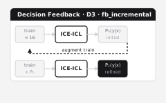
Turbo-style iteration: high-confidence predictions are added back into the context as pseudo-labels, sharpening the state. The "iced" suffix marks the complete pipeline — process finished, all phases resolved.

pseudo-labels · turbo · ICED-ICL

Why ICE?

The name earns its place — each letter maps to something real in the architecture.

ICE Protocol

In networking, ICE (Interactive Connectivity Establishment) finds a path to data through NAT barriers. ICL-through-estimation does the same: finds a path to the target function through limited observations.

In-Circuit Emulator

An ICE attaches to a live system and observes without modifying it. The identification phase scans training rows and builds state — read-only, no updates to the data it observes.

Break the Ice

ICL solves the cold-start problem for tabular prediction — literally breaks the ice between the model prior and the target distribution.

Ice Cores

Geology: layered record drilled sequentially through time. The SSM scan passes through training rows one by one — same idea, same ordering dependency.

Crystal Structure

Ice is transparent, crystalline. The model crystallises a compact, structured representation of the data from what looked like a self-attention soup.

Ice Cold

“What’s cooler than being cool?” — zero overfitting, regularised through a bottleneck state, no spurious correlations from full row-to-row attention.

Support / Cite

Contributions and citations both welcome.

Contributions

Bug reports, feature requests, and merge requests welcome at the project repository. Open an issue if you are unsure.

Citation

If you use ICE-ICL, please cite using the BibTeX entry in CITATION.cff. A JOSS submission is planned for v0.2.